Introduction to Bimachines
Bimachines are deterministic finite-state devices that represent the class regular string functions and are commonly used for text rewriting. What is fascinating about them is that they process the input text in both directions - from left to right (→) and from right to left (←) which makes them very efficient in practice as they guarantee linear time input processing.
Bimachines have less expressive power that the finite-state transducers (FST) because FSTs can also model the class of regular relations (for one input we may have more that one output). FSTs, however, are generally non-deterministic, which means that, unlike bimachines, they might not be as efficient. Unlike finite automata, not every non-deterministic transducer can be converted to an equivalent deterministic one. Also, deterministic FSTs are not powerful enough to cover the class of regular functions, so bimachines stand in-between.
In practice, when implementing algorithms, we are typically more interested in deterministic outputs, which makes the bimachines suitable for a variety of tasks due to also their high performance. In this article, we’ll introduce the concept of a bimachine and see how they work.
Bimachines
A classical bimachine is a triple \( \mathcal{B} = \langle \mathcal{A}_L, \mathcal{A}_R, \psi \rangle \), where \( \mathcal{A}_L, \mathcal{A}_R \) are deterministic finite automata and \( \psi: Q_L \times \Sigma \times Q_R \to \Sigma^* \) is called the output function of the bimachine which given a state of the left automaton, an input symbol and a state of the right automaton, it returns a string. The left automaton of the bimachine scans the text from left to right, whereas the right automaton scans from right to left. Once we get the two paths, we construct the output by concatenating the results of the output function.
Example 1
Let’s go through an example. We have the simple regular string relation \( R_1 = \{ \langle a, x \rangle, \langle ab, y \rangle \} \). What is represents is two text rewritings - either a gets replaced by x or ab gets replaced by y. This s a regular string function which can be expressed as a bimachine (Figure 1.1).
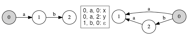
Figure 1.1: Bimachine representing R1
Note that the right and left automata’s all states are final, \(\epsilon\) represents the empty string. There are two possible successful simulations of the bimachine - one for the word a and one for the word ab.
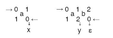
The top row depicts the recognition path in the left automaton while the text is being scanned from left to right, whereas the bottom row is the path of the right automaton while reading the text in the opposite direction. In Figure 1.2 we depict the equivalent FST.
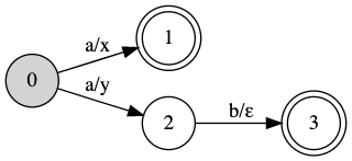
Figure 1.2: Finite-state transducer representing R1
Example 2
Let’s take a look at another example where bimachines are particularly useful. We want to mark (<, >) substrings in a text and we have the following two patterns:
a+b- a substring consists of one or more a’s followed by a ba- a substring contains the single character a
Obviously the rules overlap, so in this case we pick the longest matched substring (this makes the relation functional). Let’s mark this string relation as \( R_2 \) and see a few examples:
- \( R_2(a) = <a> \)
- \( R_2(aab) = <aab> \)
- \( R_2(baaaabba) = b<aaaab>b<a> \)
- \( R_2(aaaaa) = <a><a><a><a><a> \)
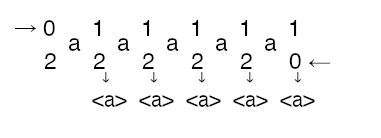
The challenge here occurs in the case where we read an a - we can either directly output <a>, or we’d have to continue reading the text until we see a b. In the case when there is no b (example 4), we’d end up reading the whole text and then backtrack all the way which would lead to \( \mathcal{O}(n^2) \) processing time. Bimachines deal with this problem quite elegantly. We construct one in Figure 2 such that it represents \( R_2 \).
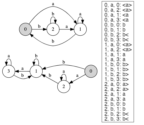
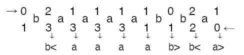
Figure 2: Bimachine representing R2
Let’s see how we process strings using this bimachine. Below the simulation of the bimachine for the input string aaaaa.
For baaaabba we end up with the following simulation.
Caveats
Bimachines are simple and efficient but, as with everything, they come at a cost. The state-of-the-art algorithms for constructing bimachines rely on building the corresponding transducer first. Due to the bimachines’ deterministic nature, we end up an upper bound of exponential time and space requirements for the construction, more specifically \( \mathcal{O}(2^{|Q|}) \) where \( |Q| \) is the number of states of the transducer. Some approaches that improve on that, given specific conditions are met, but still, the bimachine construction remains a computationally intensive operation.
The simulation procedure also requires us to store the recognition path of the right automaton while we read the text and run the left automaton. For large inputs, this might prove also costly.
Conclusion
Besides plain text rewriting, bimachines can be used for various linguistic tasks, such as text annotation, tagging, tokenization, etc. They can also be generalized in a sense that the output is in a monoid (string output is a just special type called a free monoid). Although having been around since the 1960s, even nowadays, they remain relatively unexplored. Efficient construction algorithms and applications are a good topic for further research.
References & Further Reading
- Chapters 6 - Bimachines of “Finite State Techniques - Automata, Transducers and Bimachines” by Mihov & Schulz
- A simple method for building bimachines from functional finite-state transducers by Gerdjikov, S., Mihov, S., and Schulz, K. U. (2017). In Carayol, A. and Nicaud, C., editors, Implementation and Application of Automata, pages 113–125. Springer International Publishing.
- 14.5.2 Bimachines in “Finite State Language Processing” by Roche and Schabes 1997 MIT Press
- Finite-State Transducers for Text Rewriting